Red Queen dynamics

Apr 23, 2018 12 min read Population Genetics

In this post, we will investigate how to model an evolutionary arm races, and more generally how to model a Red Queen dynamic at the population level. Diving into the population, for a specific locus in the genome, we will thus follow the life and death of alleles that are entangled into an arm race. In such arm race, the more time an allele is alive in a population, the more likely it is to die because the arm race left him lag behind, favoring new alleles that are more adapted to the environment. This life and death process of alleles can be modeled in two different regimes, a succession regime and a polymorphic regime. In the succession regime, the allele invades the population successively, so that at any given time there is only one allele in the population at the locus of interest. On the other hand, in the polymorphic regime, at any given time there are multiple alleles in the locus of interest. Because of there differences, these two regimes must be modeled very differently, but we will actually see that the results are surprisingly very similar.

We will start with the definitions and the modeling of the Red Queen dynamic, and pursue with finding solutions to the set of equations using approximations from statistical physics (the mean-field approximation). Finally we will compare our results to simulations, and also discuss the biological implications of these results.

To give a bit of context to the audience and the reasons behind the writing of this blog’s post, it is worth mentioning that this model has first been developed and published in the context of an intra-genomic Red Queen, for the specific PRDM9 locus. But since the mathematics can be applied to a more general case than the aim of the original publications, it is worth developing the mathematical material for anyone interested in modeling Red Queen dynamics.

Succession regime

To start off with definition, shamelessly copy-pasted from wikipedia, the Red Queen effect is an evolutionary hypothesis which proposes that organisms must constantly adapt, simply to survive in the ever-changing environment.

The most obvious example of this Red Queen effect is the arms races between predators and prey, where the only way predators can compensate for a better defense by the prey is by developing a better offense. Another example with well document empirical evidence is host-pathogen arm race, with a similar mechanism where the only way for a host to compensate for a better avoidance by the pathogen is to develop a better recognition. The host’s recognition mechanism is mediated by the immune system, and kinases and immunoglobulins evolve considerably faster than other proteins in the genome, empirically measured by the rate of molecular evolution of such genes.

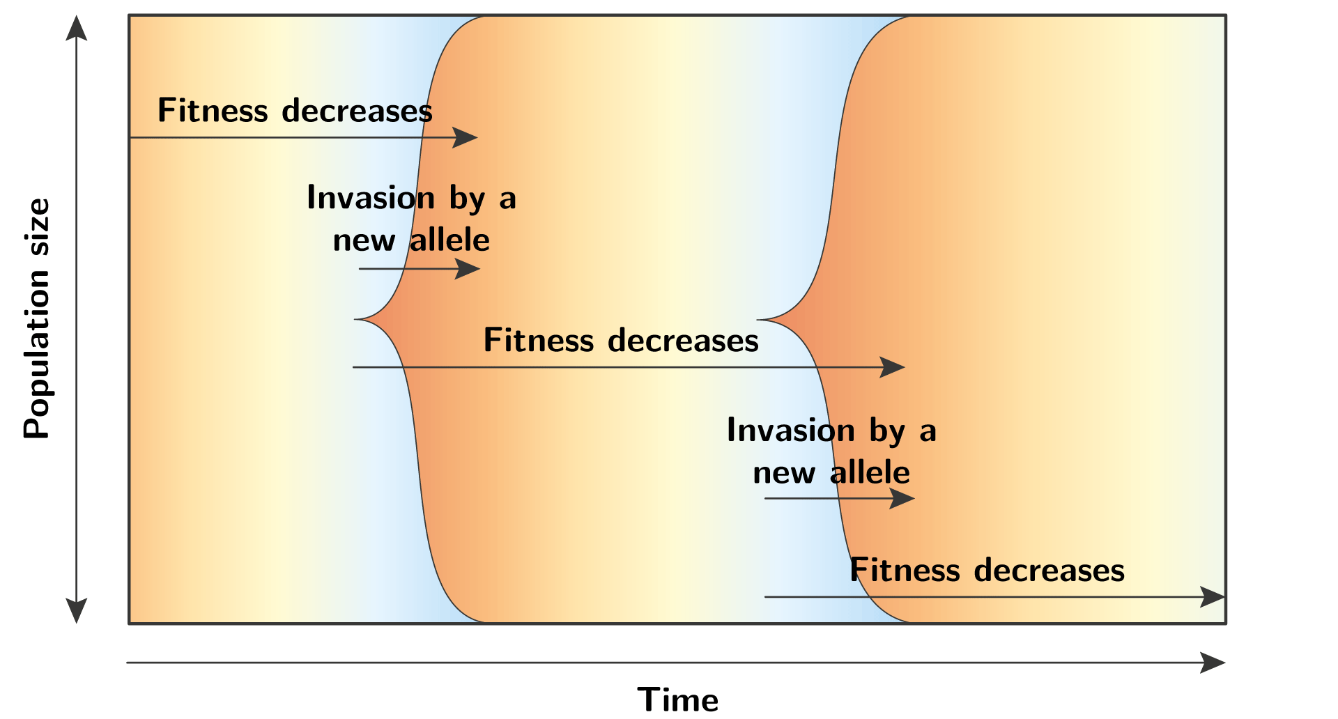
In terms of population genetics, this Red Queen dynamics can be seen as recurrent waves of allele invasion, at a specific locus. Each wave unfolds with the same mechanism, where the fitness of the resident allele decreases trough time, until a mutation creates a new allele with a better fitness, and this allele invades the population. This new allele will also see its fitness decreasing trough time, and the cycle continue again and again…

Red Queen dynamics in succession regime

Polymorphic regime

The successive waves of allele invasion is a specific case of Red Queen dynamics. More generally, it is completely possible that at any given time there are multiple alleles in the population, hence the locus of interest is polymorphic. In such polymorphic regime, a mutation that creates a new allele is not competing against the resident allele, but against the background of many residents.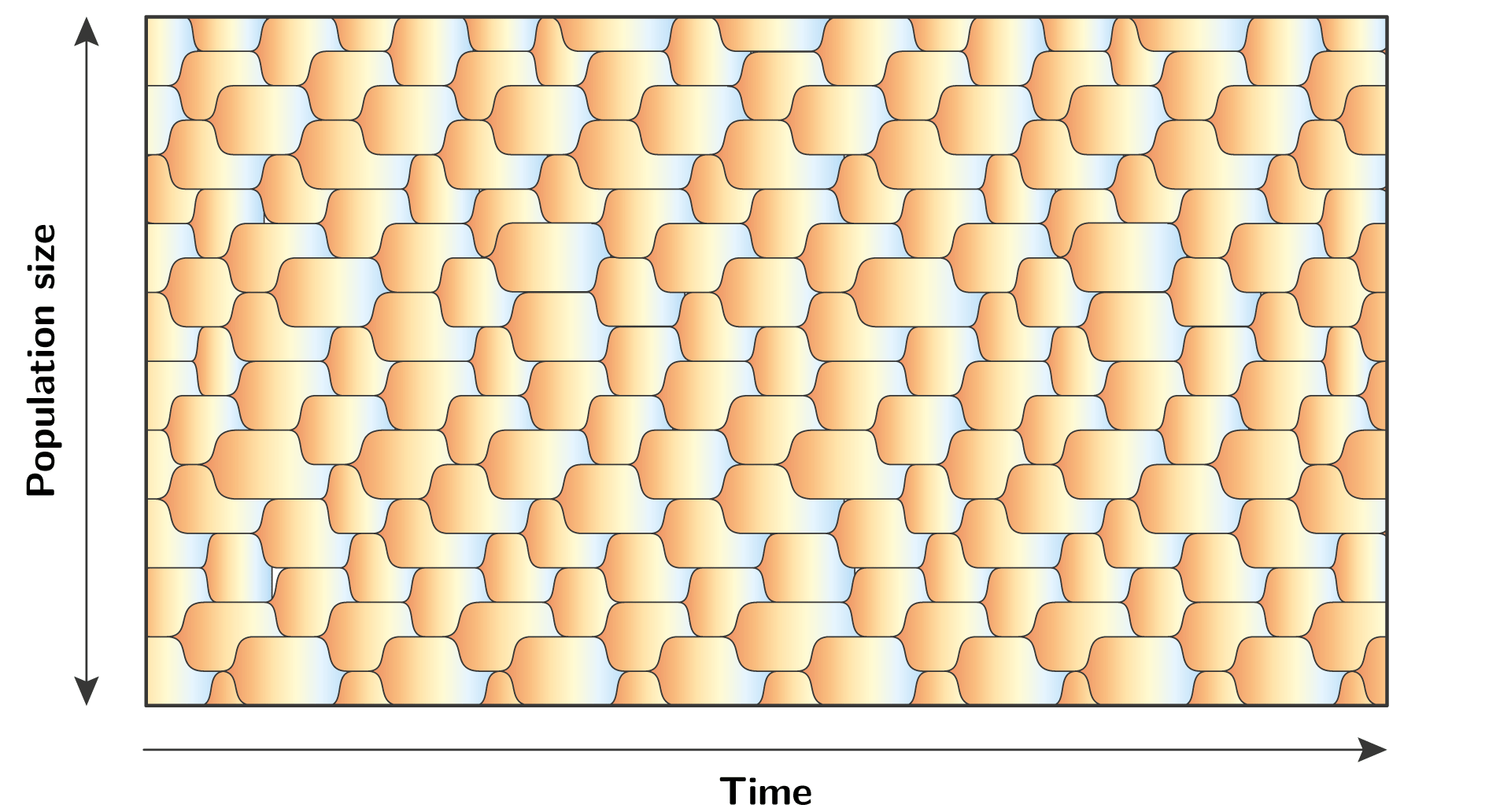 Red Queen dynamics in polymorphic regime

Equations in polymorphic regime

Now that the definitions are set, we can start with the model and delve ourselves into the equations, and we will start by the case of a polymorphic regimes… seat belts on ! $\definecolor{RED}{RGB}{235,98,49} \definecolor{YELLOW}{RGB}{226,157,38} \definecolor{BLUE}{RGB}{93,128,180} \definecolor{LIGHTGREEN}{RGB}{106,189,155} \definecolor{GREEN}{RGB}{143,176,62} \definecolor{PURPLE}{RGB}{190,30,45} \definecolor{BROWN}{RGB}{169,124,80} \definecolor{PINK}{RGB}{218,28,92} $

At the specific locus of interest, we want to keep track of the fitness for each allele in the population. This fitness, for the $i^{\text{th}}$ allele at time $t$, is going to be called $\color{YELLOW}{\omega_i(t)}$, and will strictly decay trough time. Indeed the fitness decay is specific to the red-queen dynamic, since the ever-changing environment implies that an allele is less and less fit. A first assumption in our model is to consider an exponential decay of fitness, at the rate $\rho$. The assumption of exponential decay implies that the instantaneous rate of decay is proportional to the fitness of the allele:

$$ \forall i\text{, } \dfrac{\text{d} \color{YELLOW}{\omega_i(t)} }{\text{d} t} = - \rho \color{YELLOW}{\omega_i(t)}. $$

This equation is definitively not satisfactory, because it doesn’t take into the frequency of this allele, a variable that we are going to call $\color{BLUE}{x_i(t)}$. A more realistic model would consider that the fitness of an allele is going to decrease even more if the allele is at higher frequency in the population. Mathematically, this corresponds to a rate of decay proportional to the allele frequency, and our equation suddenly becomes more complex:

$$ \forall i\text{, } \dfrac{\text{d} \color{YELLOW}{\omega_i(t)} }{\text{d} t} = - \rho \color{BLUE}{x_i(t)} \color{YELLOW}{\omega_i(t)}. $$

Our system is thus more realistic, but more complex and we just can’t solve this set of equations anymore, simply because we have more unknowns than equations.

To introduce equations and hope to solve this system, we also need to model the changes of allele frequencies trought time. Fortunately, if we consider the population large enough (absence of genetic drift), the Wright-Fisher equation model the changes of allele frequencies, precisely using the allele’s fitness. The Wright-Fisher equation states that the rate of change for the allele’s frequency is proportional to the selection coefficient. The selection coefficient is the relative difference between the allele fitness and the fitness of the whole population. We are going to call $\color{GREEN}{\bar{\omega}(t)}$ the fitness of the whole population, and the the Wright-Fisher equation is:

$$ \forall{i}\text{, } \dfrac{\text{d} \color{BLUE}{x_i(t)} }{\text{d} t} = \dfrac{\color{YELLOW}{\omega_i(t)} - \color{GREEN}{\bar{\omega}(t)} }{\color{GREEN}{\bar{\omega}(t)}} \color{BLUE}{x_i(t)}, $$ where $\color{GREEN}{\bar{\omega}(t)} = \sum_{i} \color{BLUE}{x_i(t)} \color{YELLOW}{\omega_i(t)}$.

Summarizing our system of equation, for $K(t)$ alleles in the population, we have a system of $2K(t)$ equations for the changes in fitnesses and frequencies. $$ \left\{ \begin{aligned} \forall{i}\text{, } \dfrac{\text{d} \color{BLUE}{x_i(t)} }{\text{d} t} & = \dfrac{\color{YELLOW}{\omega_i(t)} - \color{GREEN}{\bar{\omega}(t)} }{\color{GREEN}{\bar{\omega}(t)}} \color{BLUE}{x_i(t)} \\
\forall i\text{, } \dfrac{\text{d} \color{YELLOW}{\omega_i(t)} }{\text{d} t} &= - \rho \color{BLUE}{x_i(t)} \color{YELLOW}{\omega_i(t)} \\
\color{GREEN}{\bar{\omega}(t)} &= \sum_{i} \color{BLUE}{x_i(t)} \color{YELLOW}{\omega_i(t)} \end{aligned} \right. $$

This system is just to complex to solve, and yet we did not introduce new alleles entering the system with mutations.

Mean-Field approximation

To get a chance to solve our system of equations, we are going to apply a mean-field approximation. Basically, to apply a mean-field approximation, we need to find a variable which have 2 characteristics :

Being a global variable, that is a function of all the other variables.
The equations must depend on each other uniquely trough this global variable.

Once we identify a global variable, the first trick of the mean-field approximation is to consider this variable as external to the system, and not a function of the other variables anymore. Staring at our system of equations long enough, we can point out a volunteer: $\color{GREEN}{\bar{\omega}(t)}$. We thus apply the mean-field approximation and call the mean fitness $\color{GREEN}{\bar{\omega}}$, not depend on time since it’s now an external parameter. The second trick of the mean-field approximation is to consider that each allele have the same trajectory, and instead of considering $K(t)$ alleles, we simply consider 1 and assume all the other have the same behavior (but with a time delay, we will come to this later). Applying the 2 tricks of mean-field approximation, our system of $2K(t)$ equations becomes a sytem of 2 equations for a focal allele:

$$ \left\{ \begin{aligned} \dfrac{\text{d} \color{BLUE}{x(t)} }{\text{d} t} & = \dfrac{\color{YELLOW}{\omega(t)} - \color{GREEN}{\bar{\omega}} }{\color{GREEN}{\bar{\omega}}} \color{BLUE}{x(t)} \\
\dfrac{\text{d} \color{YELLOW}{\omega(t)} }{\text{d} t} &= - \rho \color{BLUE}{x(t)} \color{YELLOW}{\omega(t)} \end{aligned} \right. $$

Trajectory of the focal allele

Our system of equation for a focal allele is still not analytically solvable. But we can solve this numerically, given a value of $\color{GREEN}{\bar{\omega}}$, and we get trajectories similar to the one drawn below: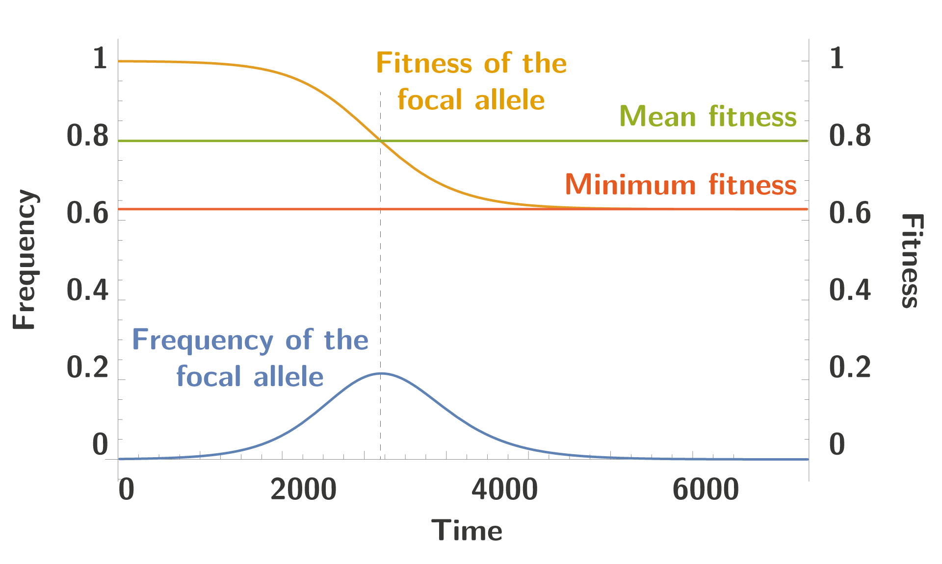 Trajectory of a focal allele

We can see the typical trajectory of the focal allele, increasing in frequency until its fitness is equal the mean fitness in the population, at which point the frequency decreases until extinction. To note the fitness doesn’t decrease up to 0, and the allele become extinct long before this event happens.

Now we have a trajectory of a focal allele, and now can start to introduce new alleles into the system with mutations.

Tilling argument

To model new alleles entering the system, we need to consider the time between two successive invasion, a variable we are going to call $\color{BROWN}{\tau}$. Under the assumption that this time $\color{BROWN}{\tau}$ is constant, we can notice a peculiar property that can be roughly described as such: looking at different alleles at one specific time is the same thing as looking at one focal allele at different time.

To better understand this property a figure is worth 1000 words: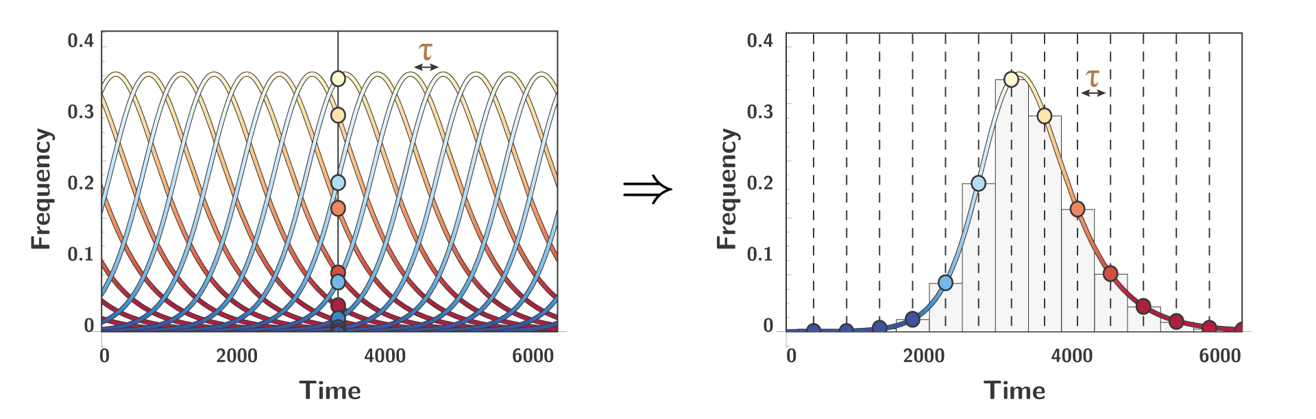 The tilling argument

Mathematically, this property translates to the following constrain on $\color{BLUE}{x(t)}$: $$ \sum_{i} \color{BLUE}{x_i(t)} \color{black} = 1 \quad \Rightarrow \quad \color{BROWN}{\tau} \color{black} \simeq \int_{0}^{\infty} \color{BLUE}{x(t)} \color{black} \text{d} t $$ Intuitively, this means that the frequency of the focal allele is constrained by the time between successive invasions. With less time between invasions, the lower the frequency that one particular allele will reach.

Thanks to this constrain, we can actually derive a mathematical relationship between $\color{GREEN}{\bar{\omega}}$ and $\color{BROWN}{\tau}$: $$ \left\{ \begin{aligned} \dfrac{\text{d} \color{BLUE}{x(t)} }{\text{d} t} & = \dfrac{\color{YELLOW}{\omega(t)} - \color{GREEN}{\bar{\omega}} }{\color{GREEN}{\bar{\omega}}} \color{BLUE}{x(t)} \\
\dfrac{\text{d} \color{YELLOW}{\omega(t)} }{\text{d} t} &= - \rho \color{BLUE}{x(t)} \color{YELLOW}{\omega(t)} \\
\color{BROWN}{\tau} \color{black} & \simeq \int_{0}^{\infty} \color{BLUE}{x(t)} \color{black} \text{d} t \end{aligned} \right. \ \Rightarrow \ \color{GREEN}{\bar{\omega}} \color{black} \simeq \dfrac{1 - e^{- \rho \color{BROWN}{\tau} }}{\rho \color{BROWN}{\tau} } $$ The mean-field approximation leads us to the conclusion that for a given mean fitness $\color{GREEN}{\bar{\omega}}$, there is only one trajectory possible for the alleles, and this means that only one time between successive invasions $\color{BROWN}{\tau}$ is acceptable.

Solving the self-consistent equation

So far, we have a relationship between $\color{GREEN}{\bar{\omega}}$ and $\color{BROWN}{\tau}$ given by the mean-field approximation. And, we now are going to develop the third and last trick of the mean-approximation… We are going to derive a self-consistent equation for $\color{GREEN}{\bar{\omega}}$ (and equivalently $\color{BROWN}{\tau}$).

We return to population genetic, and thanks to the kimura formula, the compute the probability of fixation of a new allele ($p_{fix}$), given by: $$ p_{fix} \simeq \dfrac{1 - \color{GREEN}{\bar{\omega}} }{\color{GREEN}{\bar{\omega}}}, $$

If we introduce new allele in the population at rate $\mu$, then the rate of invasion of new mutants, which is by the way the inverse of the time between sucessive invasion $\color{BROWN}{\tau}$, is given by the product of the mutation rate and the probability of fixation: $$ \color{BROWN}{\tau}^{\color{black}{-1}} \color{black} = \mu \ p_{fix} \simeq \mu \dfrac{1 - \color{GREEN}{\bar{\omega}} }{\color{GREEN}{\bar{\omega}}}, $$

Altogether, we get the self-consistent equation of $\color{GREEN}{\bar{\omega}}$ $$ \left\{ \begin{aligned} \color{GREEN}{\bar{\omega}} \color{black} & \simeq \dfrac{1 - e^{- \rho \color{BROWN}{\tau} }}{\rho \color{BROWN}{\tau} } \\
\color{BROWN}{\tau}^{\color{black}{-1}} \color{black} & \simeq \mu \dfrac{1 - \color{GREEN}{\bar{\omega}} }{\color{GREEN}{\bar{\omega}}} \end{aligned} \right. $$ $$ \Rightarrow \ \color{GREEN}{\bar{\omega}} \color{black} \simeq g\left( \color{GREEN}{\bar{\omega}} \color{black}, \dfrac{\rho}{\mu}\right) \simeq \dfrac{\mu}{\rho} \dfrac{1 - \color{GREEN}{\bar{\omega}} }{\color{GREEN}{\bar{\omega}} } \left( 1 - e^{- \dfrac{\rho}{\mu} \dfrac{ \color{GREEN}{\bar{\omega}} }{1 - \color{GREEN}{\bar{\omega}} } } \right) $$

With 1 equation and 1 variable we can now hope to solve this self-consistent equation and celebrate! Unfortunately, even is this equation is solvable numerically, we don’t have a close analytical solution in general.

Interestingly, if $\dfrac{\rho}{\mu} \ll 1$ we have the following approximation: $$\color{GREEN}{\bar{\omega}} \color{black} \simeq 1 - \sqrt{ \dfrac{\rho}{\mu} }$$

We thus see that the strongest the fitness decay rate ($\rho$), the lowest the mean fitness, this effect is due to all alleles decreasing rapidly in fitness. On the other hand, the strongest the mutation rate ($\mu$), the higher the mean fitness, this effect is due to new alleles appearing frequently, which are restoring fitness.

The square root in this equation is interesting since it shows that the effect is balanced, meaning that for example if we increase the decay rate $\rho$, we don’t decrease linearly the mean fitness because the Red Queen will partially compensate by recruiting new alleles more frequently.

Equations in the succession regime

Interestingly the mean fitness averaged over time is easily accessible in this special case of the succession regime, and we get: $$ \color{GREEN}{\bar{\omega}} \color{black} = \int_{0}^{\color{BROWN}{\tau}} \color{YELLOW}{\omega(t)} \color{black} \text{d}t = \dfrac{1 - e^{- \rho \color{BROWN}{\tau} }}{\rho \color{BROWN}{\tau} } $$

Which is the same as in polymorphic regime and thus we also have the same self-consistent equation: $$ \color{GREEN}{\bar{\omega}} \color{black} \simeq g\left( \color{GREEN}{\bar{\omega}} \color{black}, \dfrac{\rho}{\mu}\right) $$

Analytical approximation compared to simulation

We also build a Right-Fisher simulator, taking into account drift through integration of population size. And we compare the result of the simulation to the result of our approximation, which shows a good fit: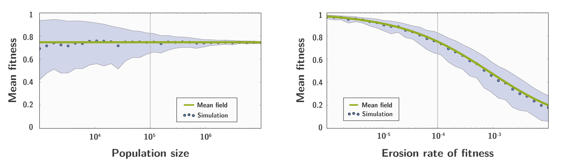 The tilling argument

Conclusion

We showed that we can solve the equation for the mean fitness of the population $\color{GREEN}{\bar{\omega}}$, and the time between successive invasions $\tau$. Moreover we showed that they are the same whenever we are in a succession or a polymorphic regime, and also we showed that they are solely a function of the ratio between mutation rate and fitness decay rate. In the polymorphic regime, we also showed that we can have the trajectory of a focal allele, and all alleles will have the same trajectory.

We have not shown it here (its more complicated, but along the line) that the diversity, meaning the effective number of alleles at the locus of interest is: $$ D = 24 N_e u $$, where $u$ is the mutation rate per locus per generation, and $N_e$ is the effective population size. This locus hence appears seemingly neutral, and the fitness decay ($\rho$) surprisingly doesn’t have any impact on the effective number of alleles.