Chronograms or Phylograms for trait evolution?
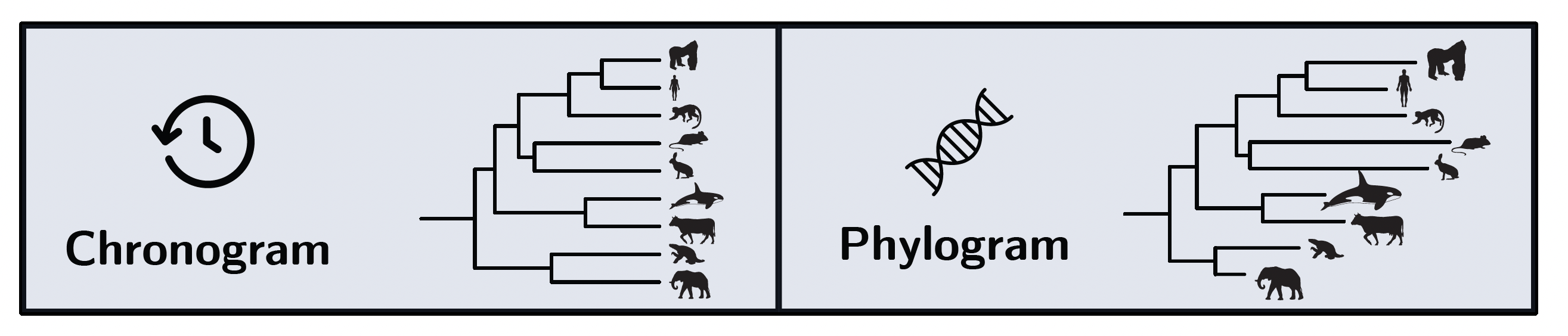
Chronograms are everywhere in evolutionary biology. Whenever a continuous trait (e.g. body size, brain mass, metabolic rate) is measured across a set of species and modelled along a phylogenetic tree, the branches of that tree are almost universally expressed in units of time. This convention rests on the intuition that elapsed time determines how much trait evolution can take place.
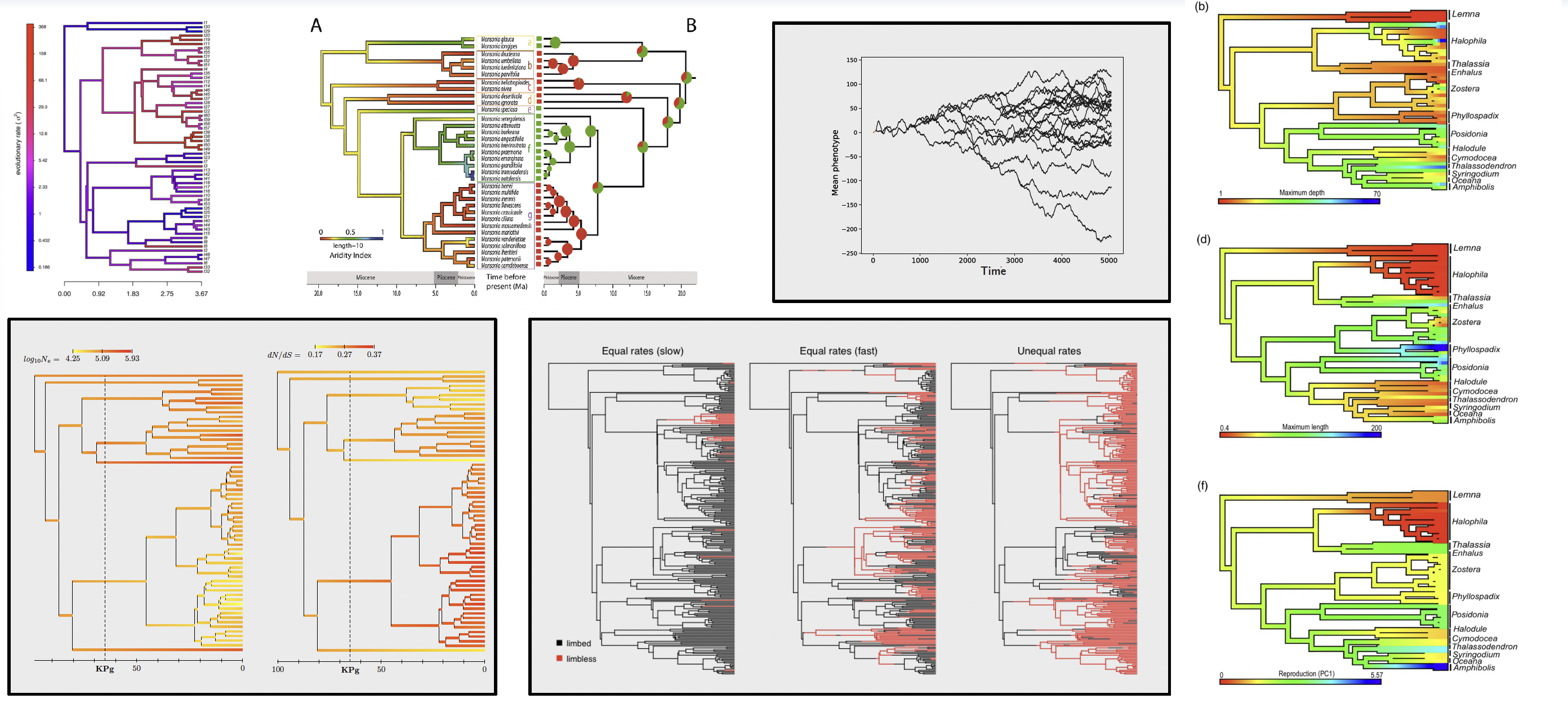
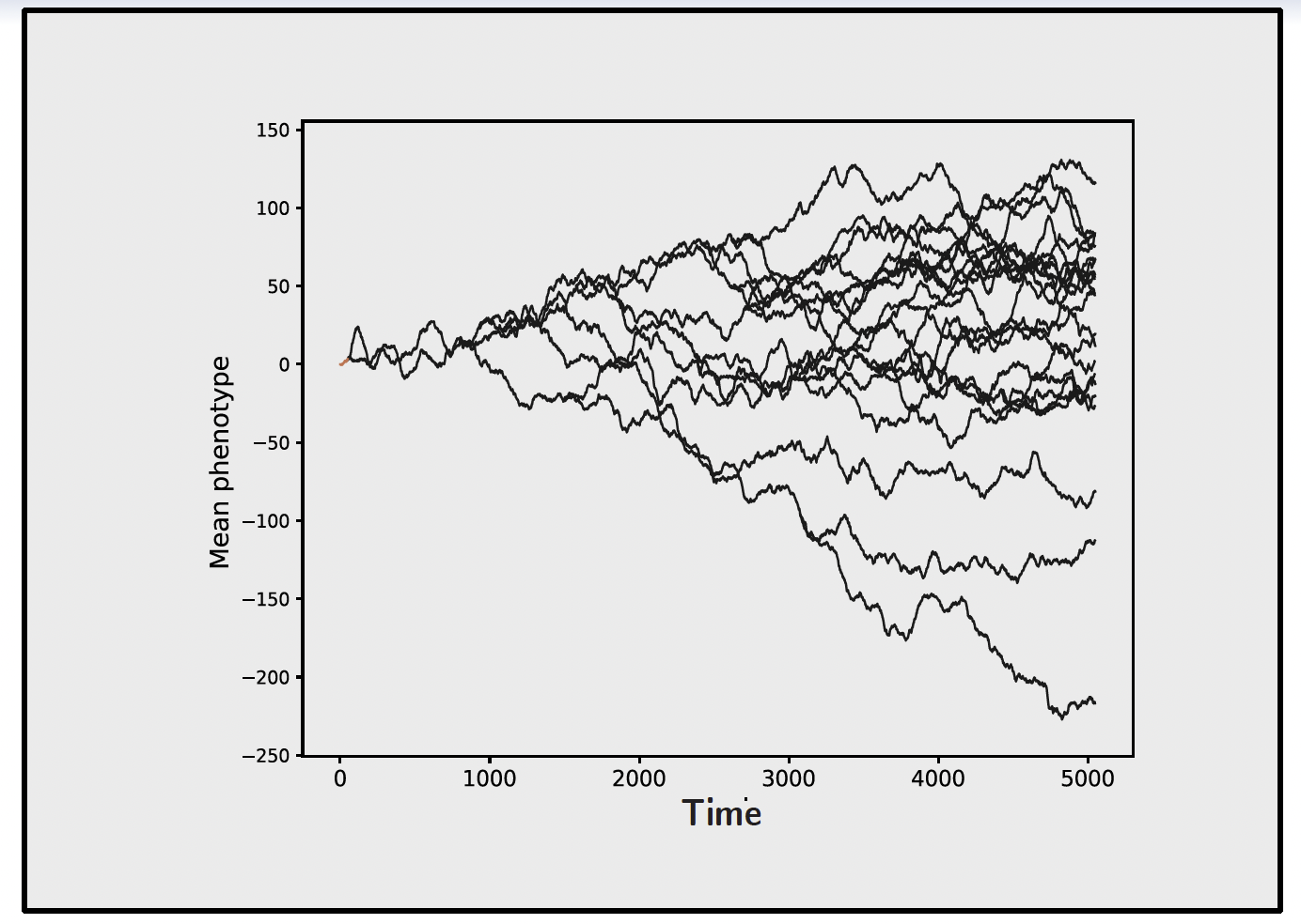
Then, to determine which evolutionary regime best explains the observed trait variation, the standard approach is to fit different models of trait evolution to the data, using the chronogram as the backbone. For examples: a Brownian motion (BM) model of neutral drift, an Ornstein-Uhlenbeck (OU) model of stabilizing selection, and a shifted OU model of directional selection. The model that best fits the data is then interpreted as the most likely evolutionary process shaping the trait across the phylogeny.
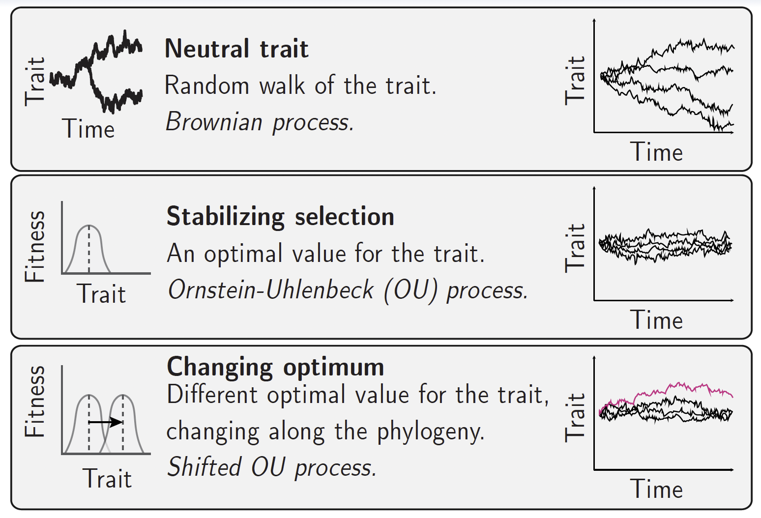
However, neutral trait evolution is not the only process that can generate a Brownian motion. If the trait is following an optimum itself moving randomly across the landscape, the trait will also perform a BM-like random walk, but one that tracks the moving optimum. In other words, a BM pattern is not proof of neutral drift; it can also arise from selection tracking a moving optimum.
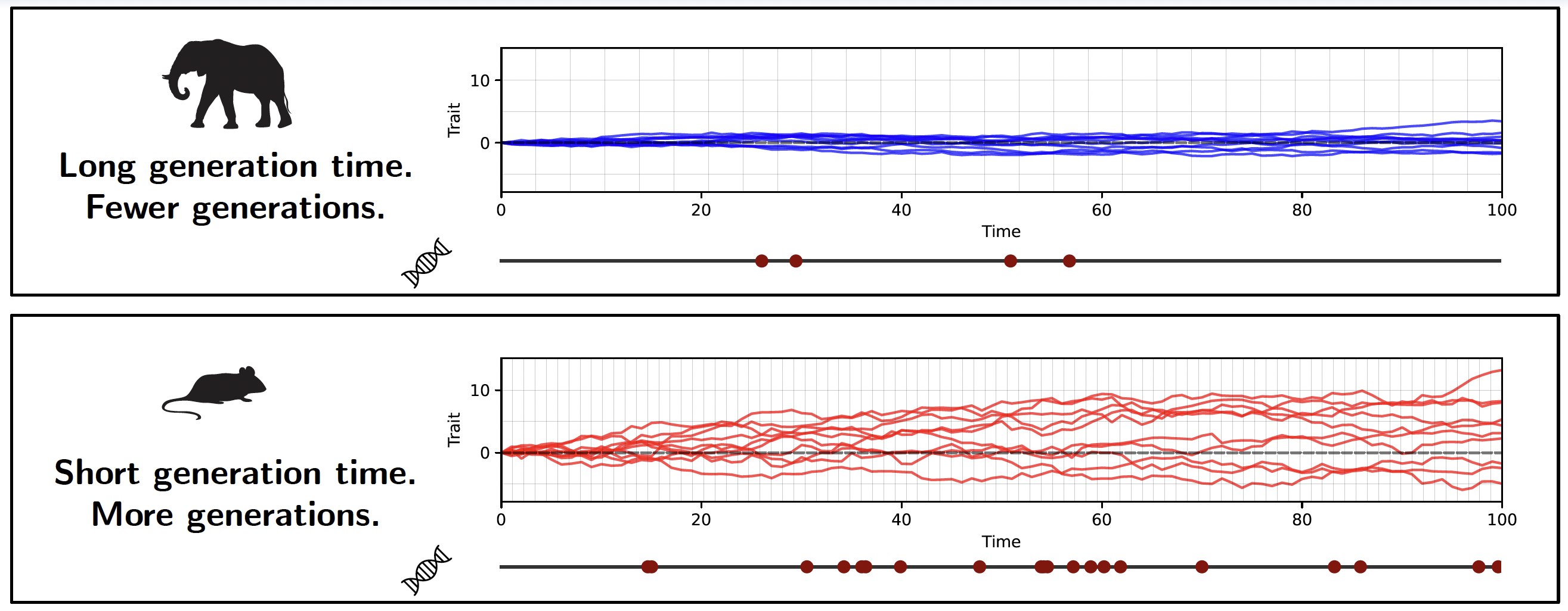
This is where the unit in which branch lengths are measured becomes crucial. If the trait is evolving neutrally, the amount of divergence between lineages depends on how many generations have passed, not on how much absolute time has elapsed. This is because neutral mutations arise and are fixed or lost on a per-generation basis (Kimura 1968). Therefore, if generation time varies across the phylogeny, a chronogram will not accurately reflect the expected divergence under neutrality. In contrast, a phylogram, where branch lengths represent nucleotide divergence at neutral genomic sites, inherently accounts for variable generation time, as it directly measures the number of neutral substitutions that have accumulated along each branch.
Thus, we can theoretically distinguish between neutral drift and selection tracking a moving optimum by comparing how well the trait data fit a BM model when using a chronogram versus a phylogram. If the trait is evolving neutrally, it should fit better on the phylogram, which accounts for generation time variation. If the trait is under selection tracking a moving optimum, it should fit better on the chronogram, which reflects elapsed time.
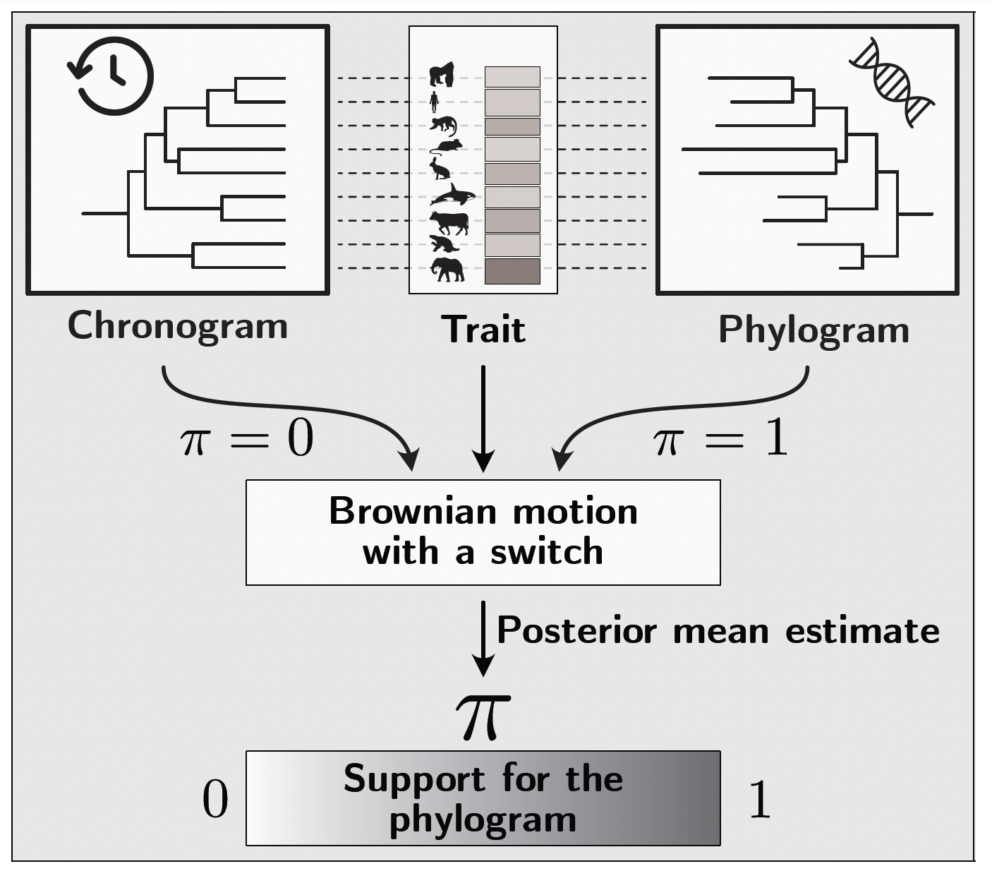
To test formally whether a trait is better described by BM running on a phylogram or on a chronogram, we developed a model with a Bayesian switch variable $\pi$. The switch is a Bernoulli variable: when $\pi = 0$, the BM is fitted using the chronogram branch lengths; when $\pi = 1$, it uses the phylogram branch lengths. Both trees are rescaled to the same total length so that the comparison is not confounded by differences in overall rate. Both trees and the trait data are provided as input, and the posterior mean of $\pi$, estimated by MCMC, gives a continuous measure of the support for the phylogram over the chronogram.
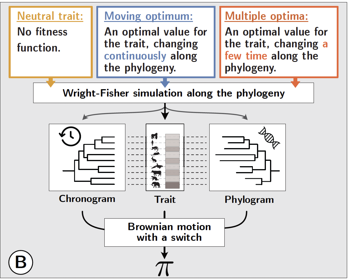
We tested this statistic using individual-based Wright-Fisher simulations along a mammalian-like phylogeny. Three evolutionary regimes were simulated: a neutral trait (flat fitness function), a trait evolving under a continuously moving optimum, and a trait under selection around multiple discrete optima. Each simulation simultaneously generated the mean trait value for extant species, the chronogram derived from the underlying time tree, and the phylogram estimated from independent neutral loci. Generation time, mutation rate, and effective population size $N_e$ were allowed to vary along the branches of the phylogeny to mimic the range of biological variation observed across mammals.
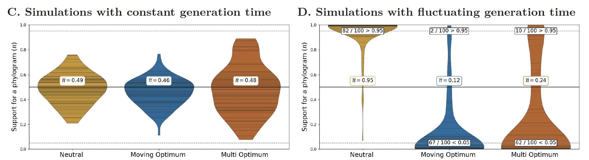
When generation time is constant across the phylogeny, the chronogram and phylogram are essentially equivalent and $\pi \approx 0.5$ regardless of the regime, as expected. When generation time varies across the tree (the biologically realistic scenario) the statistic clearly separates the regimes.
The practical implication is a refinement of standard practice in phylogenetic comparative methods. When the goal is to claim that a trait is evolving under drift, the phylogram is the appropriate backbone. Conversely, when the goal is to model and reconstruct selective regimes (e.g.) optimum shifts, rate heterogeneity) the chronogram remains the correct choice. The code to reproduce all analyses is available at github.com/ThibaultLatrille/ChronoPhylogram.